Interactive online version.
With Binder, open this notebook in an executable environment:
Rankings comparison
This tutorial provides an overview of the use of the Scikit-Criteria ranking comparison tools.
Motivation
It is interesting to note that there are many different aggregation functions (TOPSIS, WeightedSum, MOORA, etc.), which summarize multiple criteria with quite different heuristics to a single analysis dimension; if we add to this the different preprocessing (scaling, weight calculation, optimality sense transformation, etc), the approaches to compute rankings are numerous.
The question then arises:
What is the best approach MCDM is the best?
Or:
What defines that an approach is the best?
We can think of some desirable characteristics for all decision algorithms:
Be easy to understand.
That the representation of the problem is consistent.
That at the minimum change of weights everything does not change abruptly.
That any new alternative that is incorporated does not distort the ranking too much.
This ends up defining a Paradox in which
The choice of the best multi-criteria method is a multi-criteria problem.
To solve this problem we can use three different options
Compare rankings manually.
Exploiting the concept of inversion of the rankings.
Sensitivity analysis.
In this tutorial we will focus on the first option.
Tools to compare rankings manually
As of Scikit-Criteria 0.8 there is a class and a function named cmp.RanksComparator and mkrank_cmp, which consume multiple rankings and provide tools for analysis and visualization for correlation, regression and direct comparison of results.
To use them we must import them from the cmp module.
[1]:
from skcriteria.cmp import RanksComparator, mkrank_cmp
Experiment setup
First we need a dataset, lets use the decision-matrix extracted from from historical time series cryptocurrencies with windows_size=7.
[2]:
import skcriteria as skc

dm = skc.datasets.load_van2021evaluation(windows_size=7)
dm
[2]:
| xRV[▲ 1.0] | sRV[▼ 1.0] | xVV[▲ 1.0] | sVV[▼ 1.0] | xR2[▲ 1.0] | xm[▲ 1.0] | |
|---|---|---|---|---|---|---|
| ADA | 0.029 | 0.156 | 8.144000e+09 | 1.586000e+10 | 0.312 | 1.821000e-11 |
| BNB | 0.033 | 0.167 | 6.141000e+09 | 1.118000e+10 | 0.396 | 9.167000e-09 |
| BTC | 0.015 | 0.097 | 2.095000e+11 | 1.388000e+11 | 0.281 | 1.254000e-08 |
| DOGE | 0.057 | 0.399 | 8.287000e+09 | 2.726000e+10 | 0.327 | 1.459000e-12 |
| ETH | 0.023 | 0.127 | 1.000000e+11 | 8.054000e+10 | 0.313 | 1.737000e-09 |
| LINK | 0.040 | 0.179 | 6.707000e+09 | 1.665000e+10 | 0.319 | 1.582000e-09 |
| LTC | 0.015 | 0.134 | 2.513000e+10 | 1.731000e+10 | 0.320 | 1.816000e-09 |
| XLM | 0.013 | 0.176 | 4.157000e+09 | 5.469000e+09 | 0.321 | 1.876000e-11 |
| XRP | 0.014 | 0.164 | 2.308000e+10 | 2.924000e+10 | 0.322 | 7.996000e-12 |
Now let’s create three different options to evaluate our alternatives: One based on WeightedSumModel, another one based on WeightedProductModel and a final one using TOPSIS.
[3]:
from skcriteria.pipeline import mkpipe
from skcriteria.preprocessing.invert_objectives import (
    InvertMinimize,
    NegateMinimize,
)
from skcriteria.preprocessing.filters import FilterNonDominated
from skcriteria.preprocessing.scalers import SumScaler, VectorScaler
from skcriteria.agg.simple import WeightedProductModel, WeightedSumModel
from skcriteria.agg.similarity import TOPSIS

ws_pipe = mkpipe(
    InvertMinimize(),
    FilterNonDominated(),
    SumScaler(target="weights"),
    VectorScaler(target="matrix"),
    WeightedSumModel(),
)

wp_pipe = mkpipe(
    InvertMinimize(),
    FilterNonDominated(),
    SumScaler(target="weights"),
    VectorScaler(target="matrix"),
    WeightedProductModel(),
)

tp_pipe = mkpipe(
    NegateMinimize(),
    FilterNonDominated(),
    SumScaler(target="weights"),
    VectorScaler(target="matrix"),
    TOPSIS(),
)
Now let’s run the three options and visualize the rankings
[4]:
wsum_result = ws_pipe.evaluate(dm)
wprod_result = wp_pipe.evaluate(dm)
tp_result = tp_pipe.evaluate(dm)

display(wsum_result, wprod_result, tp_result)
| Alternatives | ADA | BNB | BTC | DOGE | ETH | LINK | LTC | XLM | XRP |
|---|---|---|---|---|---|---|---|---|---|
| Rank | 8 | 2 | 1 | 7 | 3 | 5 | 6 | 4 | 9 |
| Alternatives | ADA | BNB | BTC | DOGE | ETH | LINK | LTC | XLM | XRP |
|---|---|---|---|---|---|---|---|---|---|
| Rank | 6 | 2 | 1 | 9 | 3 | 5 | 4 | 7 | 8 |
| Alternatives | ADA | BNB | BTC | DOGE | ETH | LINK | LTC | XLM | XRP |
|---|---|---|---|---|---|---|---|---|---|
| Rank | 6 | 2 | 1 | 8 | 5 | 3 | 4 | 7 | 9 |
Creating a RanksComparator instance
There are two ways to create the ranks comparators:
Rither we use the
RanksComparatorclass giving a sequence[[("name0", rank0), ("name1", rank1), ..., ("nameN", rankN)]and an extra, referring to extra information about the comparator.
[5]:
RanksComparator([("ts", tp_result), ("ws", wsum_result), ("wp", wprod_result)], extra={})
[5]:
<RanksComparator [ranks=['ts', 'ws', 'wp']]>
we let the names be inferred from the methods with the
mkrank_cmp()function. In this case, the parameter “extra” wouldn’t be necessary
[6]:
rcmp = mkrank_cmp(tp_result, wsum_result, wprod_result)
rcmp
[6]:
<RanksComparator [ranks=['TOPSIS', 'WeightedSumModel', 'WeightedProductModel']]>
RankComparator utilities
A set of useful statistics is provided to compare correlations, trends and covariances between the different rankings.
We can start by looking at the correlations
[7]:
rcmp.corr() # by default the pearson correlation is used
[7]:
| Method | TOPSIS | WeightedSumModel | WeightedProductModel |
|---|---|---|---|
| Method | |||
| TOPSIS | 1.000000 | 0.783333 | 0.916667 |
| WeightedSumModel | 0.783333 | 1.000000 | 0.816667 |
| WeightedProductModel | 0.916667 | 0.816667 | 1.000000 |
[8]:
rcmp.corr(method="kendall") # or we can us the kendal correlation
[8]:
| Method | TOPSIS | WeightedSumModel | WeightedProductModel |
|---|---|---|---|
| Method | |||
| TOPSIS | 1.000000 | 0.666667 | 0.777778 |
| WeightedSumModel | 0.666667 | 1.000000 | 0.666667 |
| WeightedProductModel | 0.777778 | 0.666667 | 1.000000 |
Covariances are also available
[9]:
rcmp.cov()
[9]:
| Method | TOPSIS | WeightedSumModel | WeightedProductModel |
|---|---|---|---|
| Method | |||
| TOPSIS | 7.500 | 5.875 | 6.875 |
| WeightedSumModel | 5.875 | 7.500 | 6.125 |
| WeightedProductModel | 6.875 | 6.125 | 7.500 |
And the \(R^2\) score (the same as the linear regression) between rankings
[10]:
rcmp.r2_score()
[10]:
| Method | TOPSIS | WeightedSumModel | WeightedProductModel |
|---|---|---|---|
| Method | |||
| TOPSIS | 1.000000 | 0.566667 | 0.833333 |
| WeightedSumModel | 0.566667 | 1.000000 | 0.633333 |
| WeightedProductModel | 0.833333 | 0.633333 | 1.000000 |
Another thing available is to analyze how far one ranking is from the other.
By default the Hamming distance is used, but any of the available `scipy.spatial.distance.pdist() <https://docs.scipy.org/doc/scipy/reference/generated/scipy.spatial.distance.pdist.html#scipy.spatial.distance.pdist>`__ functions can be used.
[11]:
rcmp.distance()
[11]:
| Method | TOPSIS | WeightedSumModel | WeightedProductModel |
|---|---|---|---|
| Method | |||
| TOPSIS | 0.000000 | 0.666667 | 0.444444 |
| WeightedSumModel | 0.666667 | 0.000000 | 0.555556 |
| WeightedProductModel | 0.444444 | 0.555556 | 0.000000 |
[12]:
rcmp.distance(metric="cityblock")
[12]:
| Method | TOPSIS | WeightedSumModel | WeightedProductModel |
|---|---|---|---|
| Method | |||
| TOPSIS | 0.0 | 12.0 | 6.0 |
| WeightedSumModel | 12.0 | 0.0 | 10.0 |
| WeightedProductModel | 6.0 | 10.0 | 0.0 |
A distance function can also be provided
[13]:
def my_distance(u,v,w=None):
    return 42

rcmp.distance(metric=my_distance)
[13]:
| Method | TOPSIS | WeightedSumModel | WeightedProductModel |
|---|---|---|---|
| Method | |||
| TOPSIS | 0.0 | 42.0 | 42.0 |
| WeightedSumModel | 42.0 | 0.0 | 42.0 |
| WeightedProductModel | 42.0 | 42.0 | 0.0 |
Finally, if all this is insufficient, we can turn the comparator into a pandasDataFrame
[14]:
rcmp.to_dataframe()
[14]:
| Method | TOPSIS | WeightedSumModel | WeightedProductModel |
|---|---|---|---|
| Alternatives | |||
| ADA | 6 | 8 | 6 |
| BNB | 2 | 2 | 2 |
| BTC | 1 | 1 | 1 |
| DOGE | 8 | 7 | 9 |
| ETH | 5 | 3 | 3 |
| LINK | 3 | 5 | 5 |
| LTC | 4 | 6 | 4 |
| XLM | 7 | 4 | 7 |
| XRP | 9 | 9 | 8 |
RankComparator Plots!
The other set of analysis tools are obviously the visualization tools.
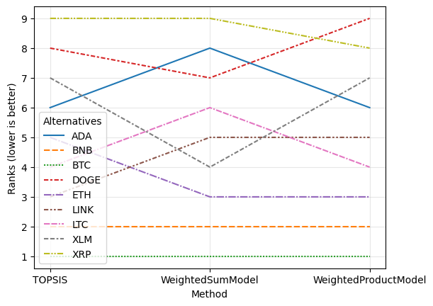
A classic in the area Ranking flows
[15]:
rcmp.plot.flow();
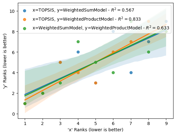
We can also run regressions on all combinations of different rankings.
[16]:
rcmp.plot.reg(r2=True, r2_fmt=".3f");
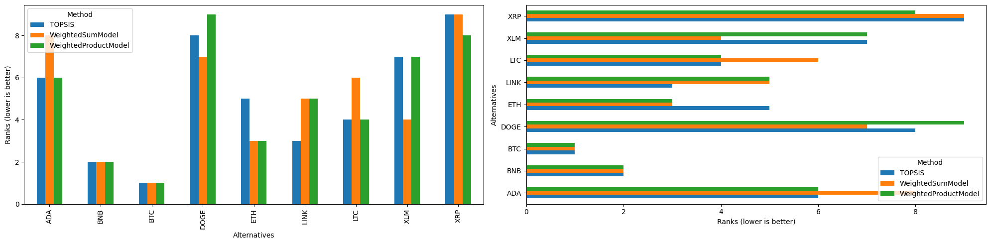
There are also bar plots
[17]:
import matplotlib.pyplot as plt

fig, axs = plt.subplots(1, 2, figsize=(20, 5))

rcmp.plot.bar(ax=axs[0])
rcmp.plot.barh(ax=axs[1])

fig.tight_layout();
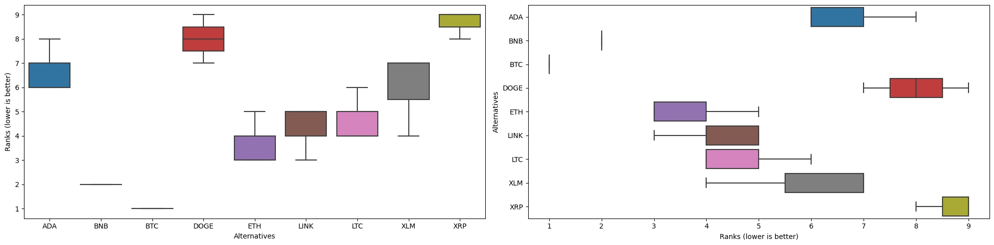
and boxplots
[18]:
fig, axs = plt.subplots(1, 2, figsize=(20, 5))

rcmp.plot.box(ax=axs[0])
rcmp.plot.box(ax=axs[1], orient="h")

fig.tight_layout();
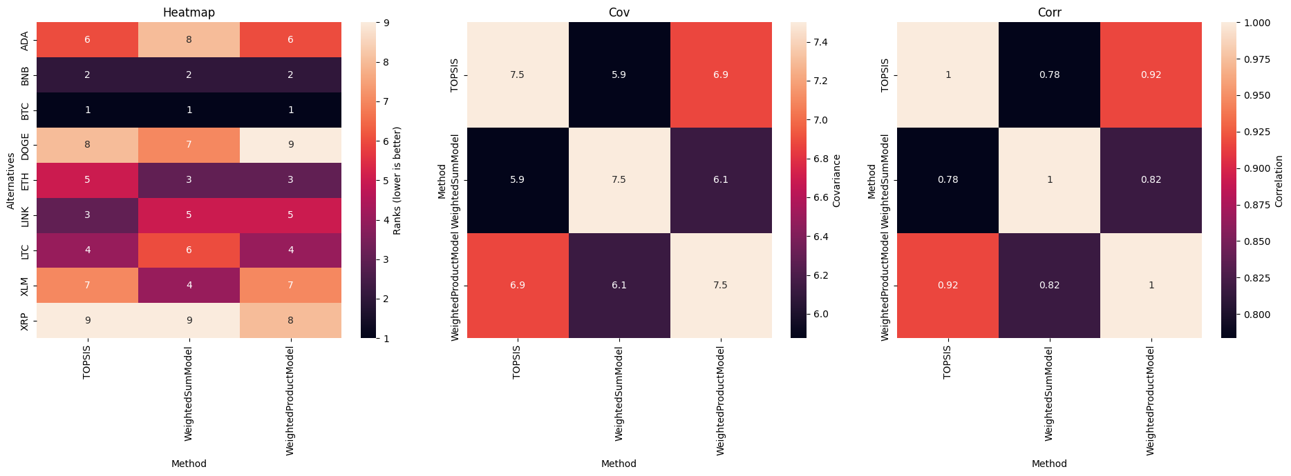
And you can visualize all matrices with statistical heatmap-like plots.
[19]:
fig, axs = plt.subplots(1, 3, figsize=(19, 7))

for kind, ax in zip(["heatmap", "cov", "corr"], axs):
    rcmp.plot(kind, ax=ax)
    ax.set_title(kind.title())


fig.tight_layout()
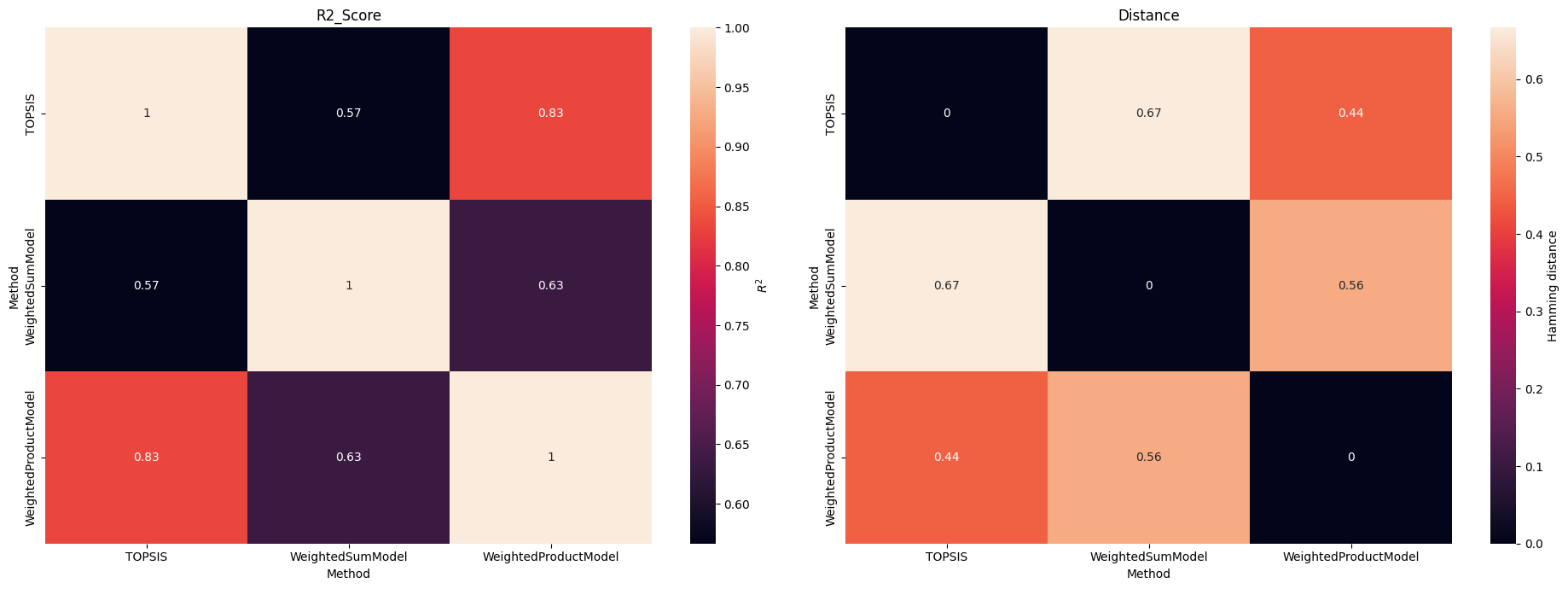
[20]:
fig, axs = plt.subplots(1, 2, figsize=(19, 7))

for kind, ax in zip(["r2_score", "distance"], axs):
    rcmp.plot(kind, ax=ax)
    ax.set_title(kind.title())

fig.tight_layout()
Generated by nbsphinx from a Jupyter notebook. 2025-08-03T00:33:12.747578