Dominance and satisfaction analysis (AKA filters)
This tutorial provides a practical overview of how to use scikit-criteria for satisfaction and dominance analysis, as well as the creation of filters for data cleaning.
Case
In order to decide to purchase a series of bonds, a company studied five candidate investments: PE, JN, AA, FX, MM and GN.
The finance department decides to consider the following criteria for selection. selection:
ROE: Return percentage. Sense of optimality, \(Maximize\).
CAP: Market capitalization. Sense of optimality, \(Maximize\).
RI: Risk. Sense of optimality, \(Minimize\).
The full decision matrix
[1]:
import skcriteria as skc

dm = skc.mkdm(
    matrix=[
        [7, 5, 35],
        [5, 4, 26],
        [5, 6, 28],
        [3, 4, 36],
        [1, 7, 30],
        [5, 8, 30],
    ],
    objectives=[max, max, min],
    alternatives=["PE", "JN", "AA", "FX", "MM", "FN"],
    criteria=["ROE", "CAP", "RI"],
)

dm
[1]:
| ROE[▲ 1.0] | CAP[▲ 1.0] | RI[▼ 1.0] | |
|---|---|---|---|
| PE | 7 | 5 | 35 |
| JN | 5 | 4 | 26 |
| AA | 5 | 6 | 28 |
| FX | 3 | 4 | 36 |
| MM | 1 | 7 | 30 |
| FN | 5 | 8 | 30 |
Satisfaction analysis
It is reasonable to think that any decision-maker would want to set “satisfaction thresholds” for each criterion, in such a way that alternatives that do not exceed the thresholds in any criterion are eliminated.
For our example we will assume that the decision-maker only accepts alternatives with \(ROE >= 2%\).
For this analysis we will need the skcriteria.preprocessing.filters module .
[2]:
from skcriteria.preprocessing import filters
The filters are transformers and works as follows:
At the moment of construction they are provided with a dict that as a key has the name of a criterion, and as a value the condition to be satisfied.
Optionally it receives a parameter
ignore_missing_criteriawhich if it is set to False (default value) fails any attempt to transform an decision matrix that does not have any of the criteria.For an alternative not to be eliminated the alternative has to pass all filter conditions.
The simplest filter consists of instances of the class filters.Filters, which as a value of the configuration dict, accepts functions that are applied to the corresponding criteria and returns a mask where the True values denote the alternatives that we want to keep.
To write the function that filters the alternatives where $ROE >= 2.
[3]:
def roe_filter(v):
    return v >= 2  # criteria are numpy.ndarray

flt =  filters.Filter({"ROE": roe_filter})
flt
[3]:
Filter(criteria_filters={'ROE': <function roe_filter at 0x7f63facdf790>}, ignore_missing_criteria=False)
However, scikit-criteria offers a simpler collection of filters that implements the most common operations of equality, inequality and inclusion a set.
In our case we are interested in the FilterGE class, where GE stands for Greater or Equal.
So the filter would be defined as
[4]:
flt = filters.FilterGE({"ROE": 2})
flt
[4]:
FilterGE(criteria_filters={'ROE': 2}, ignore_missing_criteria=False)
The way to apply the filter to a DecisionMatrix, is like any other transformer:
[5]:
dmf = flt.transform(dm)
dmf
[5]:
| ROE[▲ 1.0] | CAP[▲ 1.0] | RI[▼ 1.0] | |
|---|---|---|---|
| PE | 7 | 5 | 35 |
| JN | 5 | 4 | 26 |
| AA | 5 | 6 | 28 |
| FX | 3 | 4 | 36 |
| FN | 5 | 8 | 30 |
As can be seen, we eliminated the alternative MM which did not comply with an \(ROE >= 2\).
If on the other hand (to give an example) we would like to filter out the alternatives \(ROE > 3\) and \(CAP > 4\) (using the original matrix), we can use the filter FilterGT where GT is Greater Than.
[6]:
filters.FilterGT({"ROE": 3, "CAP": 4}).transform(dm)
[6]:
| ROE[▲ 1.0] | CAP[▲ 1.0] | RI[▼ 1.0] | |
|---|---|---|---|
| PE | 7 | 5 | 35 |
| AA | 5 | 6 | 28 |
| FN | 5 | 8 | 30 |
Note:
If it is necessary to filter the alternatives by two separate conditions, a pipeline can be used. An example of this can be seen below, where we combine a satisficing and a dominance filter
The complete list of filters implemented by Scikit-Criteria is:
filters.Filter: Filter alternatives according to the value of a criterion using arbitrary functions.filters.Filter({"criterion": lambda v: v > 1})
filters.FilterGT: Filter Greater Than (\(>\)).filters.FilterGT({"criterion": 1})
filters.FilterGE: Filter Greater or Equal than (\(>=\)).filters.FilterGE({"criterion": 2})
filters.FilterLT: Filter Less Than (\(<\)).filters.FilterLT({"criterion": 1})
filters.FilterLE: Filter Less or Equal than (\(<=\)).filters.FilterLE({"criterion": 2})
filters.FilterEQ: Filter Equal (\(==\)).filters.FilterEQ({"criterion": 1})
filters.FilterNE: Filter Not-Equal than (\(!=\)).filters.FilterNE({"criterion": 2})
filters.FilterIn: Filter if the values is in a set (\(\in\)).filters.FilterIn({"criterion": [1, 2, 3]})
filters.FilterNotIn: Filter if the values is not in a set (\(\notin\)).filters.FilterNotIn({"criterion": [1, 2, 3]})
Dominance
An alternative \(A_0\) is said to dominate an alternative \(A_1\) (\(A_0 \succeq A_1\)), if \(A_0\) is equal in all criteria and better in at least one criterion. On the other hand, \(A_0\) strictly dominate \(A_1\) (\(A_0\) \succeq `A_1$). :math:`A_1 (\(A_0 \succ A_1\)), if \(A_0\) is better on all criteria than \(A_1\).
Under this same train of thought, an alternative that dominates all others is called a “dominant alternative”. If there is a dominant alternative, it is undoubtedly the best choice, as long as a full ranking is not required.
On the other hand, an alternative is dominated if there exists at least one other alternative that dominates it. If a dominated alternative exists and a consigned ordering is not desired, it must be removed from the set of decision alternatives.
Generally only the non-dominated or efficient alternatives are the interested ones.
Scikit-Criteria dominance analysis
Scikit-criteria, contains a number of tools within the attribute, DecisionMatrix.dominance, useful for the evaluation of dominant and dominated alternatives.
For example, we can access all the dominated alternatives by using the dominated method
[7]:
dmf.dominance.dominated()
[7]:
PE    False
JN    False
AA    False
FX     True
FN    False
dtype: bool
It can be seen with this, that FX is an dominated alternative. In addition if we want to know which are the strictly dominated alternatives we need to provide the strict parameter to the method:
[8]:
dmf.dominance.dominated(strict=True)
[8]:
PE    False
JN    False
AA    False
FX     True
FN    False
dtype: bool
It can be seen that FX is strictly dominated by at least one other alternative.
If we wanted to find out which are the dominant alternatives of FX, we can opt for two paths:
List all the dominant/strictly dominated alternatives of FX using
dominator_of().
[9]:
dmf.dominance.dominators_of("FX", strict=True)
[9]:
array(['PE', 'AA', 'FN'], dtype=object)
Use
dominance()/dominance.dominance()to see the full relationship between all alternatives.
[10]:
dmf.dominance(strict=True) # equivalent to dmf.dominance.dominance()
[10]:
| PE | JN | AA | FX | FN | |
|---|---|---|---|---|---|
| PE | False | False | False | True | False |
| JN | False | False | False | False | False |
| AA | False | False | False | True | False |
| FX | False | False | False | False | False |
| FN | False | False | False | True | False |
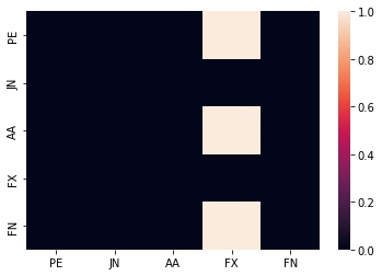
the result of the method is a DataFrame that in each cell has a True value if the row alternative dominates the column alternative.
If this matrix is very large we can, for example, visualize it in the form of a heatmap using the library seaborn
[11]:
import seaborn as sns
sns.heatmap(dmf.dominance.dominance(strict=True))
[11]:
<AxesSubplot:>
Finally we can see how each of the alternatives relate to each other dominatnes with FX using compare().
[12]:
for dominant in dmf.dominance.dominators_of("FX"):
    display(dmf.dominance.compare(dominant, 'FX'))
| Criteria | Performance | ||||
|---|---|---|---|---|---|
| ROE | CAP | RI | |||
| Alternatives | PE | True | True | True | 3 |
| FX | False | False | False | 0 | |
| Equals | False | False | False | 0 | |
| Criteria | Performance | ||||
|---|---|---|---|---|---|
| ROE | CAP | RI | |||
| Alternatives | JN | True | False | True | 2 |
| FX | False | False | False | 0 | |
| Equals | False | True | False | 1 | |
| Criteria | Performance | ||||
|---|---|---|---|---|---|
| ROE | CAP | RI | |||
| Alternatives | AA | True | True | True | 3 |
| FX | False | False | False | 0 | |
| Equals | False | False | False | 0 | |
| Criteria | Performance | ||||
|---|---|---|---|---|---|
| ROE | CAP | RI | |||
| Alternatives | FN | True | True | True | 3 |
| FX | False | False | False | 0 | |
| Equals | False | False | False | 0 | |
Filter non-dominated alternatives
Finally skcriteria offers a way to filter non-dominated alternatives, which it accepts as a parameter if you want to evaluate strict dominance.
[13]:
flt = filters.FilterNonDominated(strict=True)
flt
[13]:
FilterNonDominated(strict=True)
[14]:
flt.transform(dmf)
[14]:
| ROE[▲ 1.0] | CAP[▲ 1.0] | RI[▼ 1.0] | |
|---|---|---|---|
| PE | 7 | 5 | 35 |
| JN | 5 | 4 | 26 |
| AA | 5 | 6 | 28 |
| FN | 5 | 8 | 30 |
Full expermient
We can finally create a complete MCDA experiment that takes into account the in satisfaction and dominance analysis.
The complete experiment would have the following steps
Eliminate alternatives that do not yield at least 2% ($ROE >= $2).
Eliminate dominated alternatives.
Convert all criteria to maximize.
The weights are scaled by the total sum.
The matrix is scaled by the vector modulus.
Apply TOPSIS.
The most convenient way to do this is to use a pipeline.
[15]:
from skcriteria.preprocessing import scalers, invert_objectives
from skcriteria.madm.similarity import TOPSIS
from skcriteria.pipeline import mkpipe

pipe = mkpipe(
    filters.FilterGE({"ROE": 2}),
    filters.FilterNonDominated(strict=True),
    invert_objectives.NegateMinimize(),
    scalers.SumScaler(target="weights"),
    scalers.VectorScaler(target="matrix"),
    TOPSIS(),
)

pipe
[15]:
SKCPipeline(steps=[('filterge', FilterGE(criteria_filters={'ROE': 2}, ignore_missing_criteria=False)), ('filternondominated', FilterNonDominated(strict=True)), ('negateminimize', NegateMinimize()), ('sumscaler', SumScaler(target='weights')), ('vectorscaler', VectorScaler(target='matrix')), ('topsis', TOPSIS(metric='euclidean'))])
We now apply the pipeline to the original data
[16]:
pipe.evaluate(dm)
[16]:
| PE | JN | AA | FN | |
|---|---|---|---|---|
| Rank | 3 | 4 | 2 | 1 |
[17]:
import datetime as dt
import skcriteria

print("Scikit-Criteria version:", skcriteria.VERSION)
print("Running datetime:", dt.datetime.now())
Scikit-Criteria version: 0.7dev0
Running datetime: 2022-04-10 21:06:10.855758