Quick Start

This tutorial show how to create a scikit-criteria Data structure, and how to feed them inside different multicriteria decisions algorithms.

Conceptual Overview

The multicriteria data are really complex thing; mostly because you need at least 2 totally disconected vectors to decribe your problem: A alternative matrix (mtx) and a vector that indicated the optimal sense of every criteria (criteria); also maybe you want to add weights to your criteria

The skcteria.Data object need at least the first two to be created and also accepts the weights, the names of the criteria and the names of alternatives as optional parametes.

Your First Data object

First we need to import the Data structure and the MIN, MAX contants from scikit-criteria:

from skcriteria import Data, MIN, MAX

Then we need to create the mtx and criteria vectors.

The mtx must be a 2D array-like where every column is a criteria, and every row is an alternative

# 2 alternatives by 3 criteria
mtx = [
    [1, 2, 3],  # alternative 1
    [4, 5, 6],  # alternative 2
]
mtx

[[1, 2, 3], [4, 5, 6]]

The criteria vector must be a 1D array-like with number of elements same as number of columns in the alternative matrix (mtx). Every component of the criteria vector represent the optimal sense of each criteria.

# let's says the first two alternatives are
# for maximization and the last one for minimization
criteria = [MAX, MAX, MIN]
criteria

[1, 1, -1]

as you see the MAX and MIN constants are only aliases for the numbers -1 (minimization) and 1 (maximization). As you can see the constants usage makes the code more readable. Also you can use as aliases of minimization and maximization the built-in function min, max, the numpy function np.min, np.max, np.amin, np.amax, np.nanmin, np.nanmax and the strings min, minimization, max and maximization.

Now we can combine this two vectors in our scikit-criteria data.

# we use the built-in function as aliases
data = Data(mtx, [min, max, min])
data

ALT./CRIT.	C0 (min)	C1 (max)	C2 (min)
A0	1	2	3
A1	4	5	6

As you can see the output of the Data structure is much more friendly than the plain python lists.

To change the generic names of the alternatives (A0 and A1) and the criteria (C0, C1 and C2); let’s assume that our Data is about cars (car 0 and car 1) and their characteristics of evaluation are autonomy (MAX), comfort (MAX) and price (MIN).

To feed this information to our Data structure we have the params: anames that accept the names of alternatives (must be the same number as the rows that mtx has), and cnames the criteria names (must have same number of elements with the columns that mtx has)

data = Data(mtx, criteria,
            anames=["car 0", "car 1"],
            cnames=["autonomy", "comfort", "price"])
data

ALT./CRIT.	autonomy (max)	comfort (max)	price (min)
car 0	1	2	3
car 1	4	5	6

In our final step let’s assume we know in our case, that the importance of the autonomy is the 50%, the comfort only a 5% and the price is 45%. The param to feed this to the structure is called weights and must be a vector with the same elements as criterias on your alternative matrix (number of columns)

data = Data(mtx, criteria,
            weights=[.5, .05, .45],
            anames=["car 0", "car 1"],
            cnames=["autonomy", "comfort", "price"])
data

ALT./CRIT.	autonomy (max) W.0.5	comfort (max) W.0.05	price (min) W.0.45
car 0	1	2	3
car 1	4	5	6

Manipulating the Data

The data object are immutable, if you want to modify it you need create a new one. All the numerical data (mtx, criteria, and weights) are stored as numpy arrays, and the alternative and criteria names as python tuples.

You can acces to the different parts of your data, simply by typing data.<your-parameter-name> for example:

data.mtx

array([[1, 2, 3],
       [4, 5, 6]])

data.criteria

array([ 1,  1, -1])

data.weights

array([0.5 , 0.05, 0.45])

data.anames, data.cnames

(('car 0', 'car 1'), ('autonomy', 'comfort', 'price'))

If you want (for example) change the names of the cars from car 0 and car 1; to VW and Ford you must copy from your original Data

data = Data(data.mtx, data.criteria,
            weights=data.weights,
            anames=["VW", "Ford"],
            cnames=data.cnames)
data

ALT./CRIT.	autonomy (max) W.0.5	comfort (max) W.0.05	price (min) W.0.45
VW	1	2	3
Ford	4	5	6

Note: A more flexible data manipulation API will relased in future versions.

Plotting

The Data structure suport some basic rutines for ploting. Actually 5 types of plots are supported:

• Radar Plot (radar).
• Histogram (hist).
• Violin Plot (violin).
• Box Plot (box).
• Scatter Matrix (scatter).

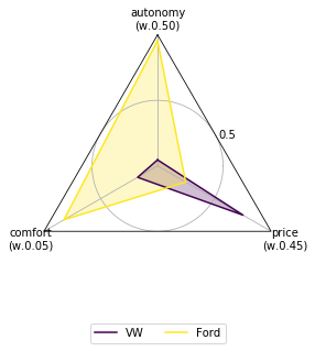
The default scikit criteria uses the Radar Plot to visualize all the data. Take in account that the radar plot by default convert all the minimization criteria to maximization and push all the values to be greater than 1 (obviously all this options can be overided).

data.plot();

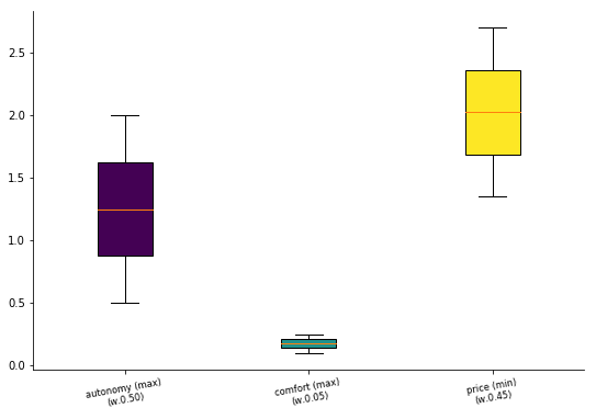
You can accesing the different plot by passing as first parameter the name of the plot

data.plot("box");

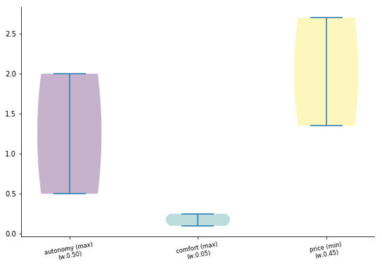
or by using the name as method call inside the plot attribute

data.plot.violin();

Every plot has their own set of parameters, but at last every one can receive:

• ax: The plot axis.
• cmap: The color map (More info).
• mnorm: The normalization method for the alternative matrix as string (Default: "none").
• wnorm: The normalization method for the criteria array as string (Default: "none").
• weighted: If you want to weight the criteria (Default: True).
• show_criteria: Show or not the criteria in the plot (Default: True in all except radar).
• min2max: Convert the minimization criteria into maximization one (Default: False in all except radar).
• push_negatives: If a criteria has values lesser than 0, add the minimun value to all the criteria (Default: False in all except radar).
• addepsto0: If a criteria has values equal to 0, add an \(\epsilon\) value to all the criteria (Default: False in all except radar).

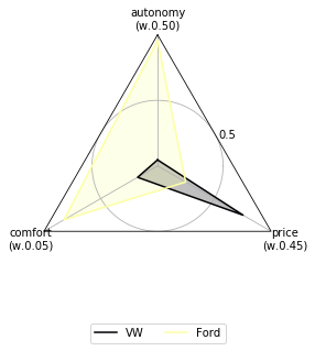
Let’s change the colors of the radar plot and show their criteria optimization sense:

data.plot.radar(cmap="inferno", show_criteria=False);

Using this data to feed some MCDA methods

Let’s rank our dummy data by Weighted Sum Model, Weighted Product Model and TOPSIS

from skcriteria.madm import closeness, simple

First you need to create the decision maker.

Most of methods accepts hyper parameters (parameters of the to configure the method) as following: 1. the method of normalization of the alternative matrix - in Weighted Sum and Weighted Product we use divided by the sum normalization - in Topsis we can also use the vector normalization 2. the method to normalize the weight array (normally sum); But complex methods has more.

Weighted Sum Model:

# first create the decision maker
# (with the default hiper parameters)
dm = simple.WeightedSum()
dm

<WeightedSum (mnorm=sum, wnorm=sum)>

# Now lets decide the ranking
dec = dm.decide(data)
dec

WeightedSum (mnorm=sum, wnorm=sum) - Solution:

ALT./CRIT.	autonomy (max) W.0.5	comfort (max) W.0.05	price (min) W.0.45	Rank
VW	1	2	3	1
Ford	4	5	6	2

The result says that the VW is better than the FORD, lets make the maths:

Note: The last criteria is for minimization and because the WeightedSumModel only accepts maximization criteria by default, scikit-criteria invert all the values to convert the criteria to maximization

print("VW:", 0.5 * 1/5. + 0.05 * 2/7. + 0.45 * 1 / (3/9.))
print("FORD:", 0.5 * 4/5. + 0.05 * 5/7. + 0.45 * 1 / (6/9.))

VW: 1.4642857142857144
FORD: 1.1107142857142858

If you want to acces this points, the Decision object stores all the particular information of every method in a attribute called e_

print(dec.e_)
dec.e_.points

Extra(points)

array([1.46428571, 1.11071429])

Also you can acces the type of the solution

print("Generate a ranking of alternatives?", dec.alpha_solution_)
print("Generate a kernel of best alternatives?", dec.beta_solution_)
print("Choose the best alternative?", dec.gamma_solution_)

Generate a ranking of alternatives? True
Generate a kernel of best alternatives? False
Choose the best alternative? True

The rank as numpy array (if this decision is a \(\alpha\)-solution / alpha solution)

dec.rank_

array([1, 2])

The index of the row of the best alternative (if this decision is a \(\gamma\)-solution / gamma solution)

dec.best_alternative_, data.anames[dec.best_alternative_]

(0, 'VW')

And the kernel of the non supered alternatives (if this decision is a \(\beta\)-solution / beta solution)

# this return None because this
# decision is not a beta-solution
print(dec.kernel_)

None

Weighted Product Model

dm = simple.WeightedProduct()
dm

<WeightedProduct (mnorm=sum, wnorm=sum)>

dec = dm.decide(data)
dec

WeightedProduct (mnorm=sum, wnorm=sum) - Solution:

ALT./CRIT.	autonomy (max) W.0.5	comfort (max) W.0.05	price (min) W.0.45	Rank
VW	1	2	3	2
Ford	4	5	6	1

As before let’s do the math (remember the weights are now exponents)

print("VW:", ((1/5.) ** 0.5) * ((2/7.) ** 0.05) + ((1 / (3/9.)) ** 0.45))
print("FORD:", ((4/5.) ** 0.5) * ((5/7.) ** 0.05) + ((1 / (6/9.)) ** 0.45))

VW: 2.059534375567646
FORD: 2.07967086650222

As wee expected the Ford are little better than the VW. Now lets theck the e_ object

print(dec.e_)
dec.e_.points

Extra(points)

array([-0.16198384,  0.02347966])

As you note the points are differents, this is because internally to avoid undeflows Scikit-Criteria uses a sums of logarithms instead products. So let’s check

import numpy as np
print("VW:", 0.5 * np.log10(1/5.) + 0.05 * np.log10(2/7.) + 0.45 * np.log10(1 / (3/9.)))
print("FORD:", 0.5 * np.log10(4/5.) + 0.05 * np.log10(5/7.) + 0.45 * np.log10(1 / (6/9.)))

VW: -0.16198383976167505
FORD: 0.023479658287116456

TOPSIS

dm = closeness.TOPSIS()
dm

<TOPSIS (mnorm=vector, wnorm=sum)>

dec = dm.decide(data)
dec

TOPSIS (mnorm=vector, wnorm=sum) - Solution:

ALT./CRIT.	autonomy (max) W.0.5	comfort (max) W.0.05	price (min) W.0.45	Rank
VW	1	2	3	2
Ford	4	5	6	1

The TOPSIS add more information into the decision object.

print(dec.e_)
print("Ideal:", dec.e_.ideal)
print("Anti-Ideal:", dec.e_.anti_ideal)
print("Closeness:", dec.e_.closeness)

Extra(ideal, anti_ideal, closeness)
Ideal: [0.48507125 0.04642383 0.20124612]
Anti-Ideal: [0.12126781 0.01856953 0.40249224]
Closeness: [0.35548671 0.64451329]

Where the ideal and anti_ideal are the normalizated sintetic better and worst altenatives created by TOPSIS, and the closeness is how far from the anti-ideal and how closer to the ideal are the real alternatives

Finally we can change the normalization criteria of the alternative matric to sum (divide every value by the sum opf their criteria) and check the result:

dm = closeness.TOPSIS(mnorm="sum")
dm

<TOPSIS (mnorm=sum, wnorm=sum)>

dm.decide(data)

TOPSIS (mnorm=sum, wnorm=sum) - Solution:

ALT./CRIT.	autonomy (max) W.0.5	comfort (max) W.0.05	price (min) W.0.45	Rank
VW	1	2	3	2
Ford	4	5	6	1

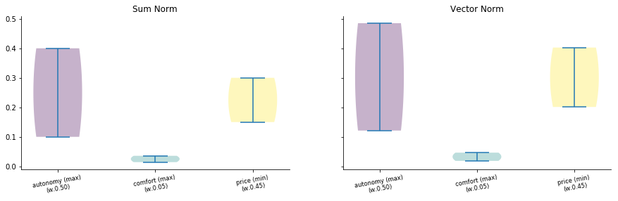
The rankin has changed so, we can compare the two normalization by plotting

import matplotlib.pyplot as plt

f, (ax1, ax2) = plt.subplots(1, 2, sharey=True)
ax1.set_title("Sum Norm")
data.plot.violin(mnorm="sum", ax=ax1);

ax2.set_title("Vector Norm")
data.plot.violin(mnorm="vector", ax=ax2);
f.set_figwidth(15)

import datetime as dt
import skcriteria
print("Scikit-Criteria version:", skcriteria.VERSION)
print("Running datetime:", dt.datetime.now())

Scikit-Criteria version: 0.2.10
Running datetime: 2019-08-27 19:49:24.273132